Walkthrough: Integrating Multiple Feature Types into a Geodatabase
In this section we will integrate data of several different formats into a single database: an Esri geodatabase used commonly in GIS applications.
This walkthrough will reiterate procedures from the previous exercises, in addition to showing how to write multiple feature types using a single writer. After integrating the data into a single database, we will carry out some basic analysis of the data.
1) Start Workbench
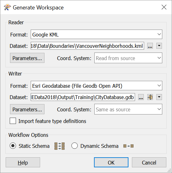
Use the Generate Workspace dialog to create a workspace using these parameters:
| Reader Format | Google KML |
| Reader Dataset | C:\FMEData2018\Data\Boundaries\VancouverNeighborhoods.kml |
| Writer Format | Esri Geodatabase (File Geodb Open API) |
| Writer Dataset | C:\FMEData2018\Output\Training\CityDatabase.gdb |
Note: Make sure you select File Geodb Open API for your geodatabase format or you may run into problems later on. The Open API implementation of GDB will allow you to create and view this geodatabase in FME Data Inspector without an Esri license. However, you will require a licensed copy of ArcMap, ArcGIS Pro, or ArcGIS Online to view the GDB in its native software. Alternatively, your instructor might ask you to use a different format, e.g., a PostGIS database; FME makes it easy to write whatever format you want.
Your dialog should look like this:
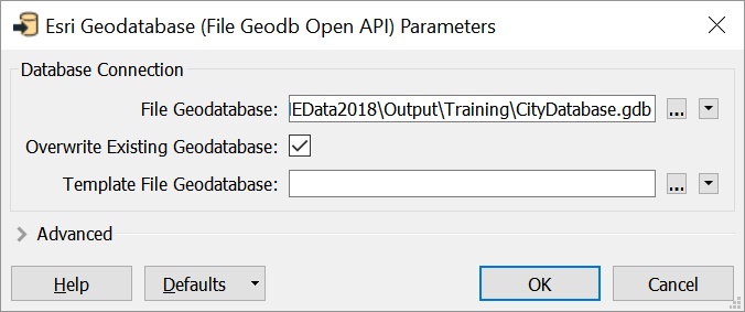
Click the Parameters buttons in the Generate Workspace dialog to check the reader/writer parameters. We will change one for this exercise. Under your Writer Parameters, in the Database Connections section, check Overwrite Existing Geodatabase. With that checked we will recreate the database entirely every time we write out the data. Your dialog should look like this:
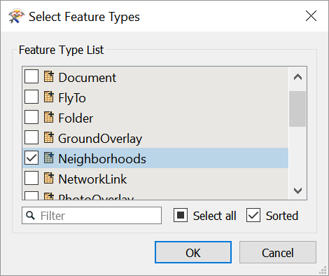
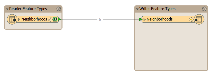
Click OK twice. You will be presented with a Select Feature Types dialog because our reader data set contains multiple layers. We only need the feature type named Neighborhoods, which contains the polygons of neighborhood boundaries. Make sure Neighborhoods is the only feature type selected:
Click OK.
Note: if you pressed OK before setting Writer Parameters, you can change this after generating your workspace. In the Navigator window under your CityDatabase FILEGDB writer > Parameters > Overwrite Existing Database (set to Yes).
2) Clean Up Generated Workspace
The generated workspace added a geometry filter automatically. This happens because Esri geodatabases store layers with only one geometry type.
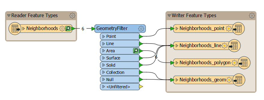
However, our reader feature type only contains polygons, so we can clean up the starting workspace by:
- deleting the GeometryFilter
- deleting the Neighborhoods_point, Neighborhoods_line, and Neighborhoods_geom writer feature types
- renaming the Neighborhoods_polygon writer feature type to just "Neighborhoods"
Your workspace should now look like this:
3) Add Excel Reader
Let's add two more readers. We'll look at two datasets from the list above that need changes to the defaults to work as we wish. Other situations that might require similar changes are covered in the Additional Procedures section.
You can add readers by clicking Readers > Add Reader, or by clicking an empty space on the canvas and typing the name or file extension of the format you wish to add and picking it from the Quick Add Menu.
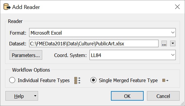
First, let's add an Excel file of public art:
| Reader Format | Microsoft Excel |
| Reader Dataset | C:\FMEData2018\Data\Culture\PublicArt.xlsx |
We will make two changes to the reader defaults.
First, change Workflow Options from Individual Feature Types (the default) to Single Merged Feature Type. The Excel reader treats rows as features and worksheets as feature types. This means by default, FME would try to read every sheet in the file as a separate feature type. If you inspect the data, you'll find it has one sheet per neighborhood. This works in Excel, but we would prefer that our database treat all the public art as one point layer. Choosing Single Merged Feature Type does this for us.
Second, we need to add a coordinate system. The reader has latitude and longitude coordinates in the Excel file, but because Excel does not store coordinate system information, we have to tell FME which one to use. We know that it is LL84, so type that into the Coordinate System box in your dialog.
Your dialog should look like this:
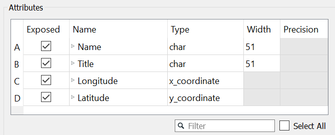
Before clicking OK, click on Parameters. We have to ensure the Reader recognizes the right columns in the Excel sheet as coordinates. Under the Attributes table column C named Longitude should by type x_coordinate and column D named Latitude should be type y_coordinate. Your dialog should look like this:
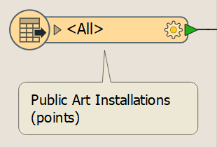
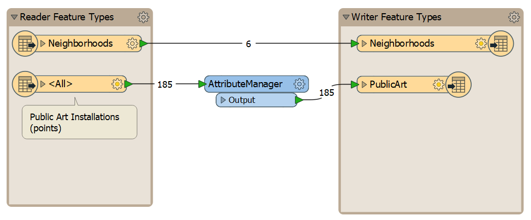
Click OK twice. This adds a new Excel reader to our Navigator window and gives it a feature type on our canvas named <All>, the default name for merged feature types. This isn't very descriptive, however. Let's add an annotation to indicate that this is the merged public art data. Right-click your feature type and select Attach Annotation. You can write something like, "Public Art Installations (points)":
Even though we added the public art installations from all neighborhoods, we can still distinguish between neighborhoods through the fme_feature_type attribute. This attribute simply gives the name of the feature type the feature belongs to. It exists on all FME features, but is not always exposed. It is exposed by default whenever you add a merged feature type. You can see it if you click the drop-down arrow next to your new <All> reader feature type.
If you right-click this feature type and select Inspect you can see that the data is still organized by neighborhood. If you select a feature the first attribute shown in the Feature Information window is FME Feature Type, which gives the neighborhood name.
Let's turn that fme_feature_type attribute into something more meaningful for our geodatabase. Add an AttributeManager after the <All> reader feature type. Open the Parameter Editor and click in the Attribute Actions table in the Output Attributes column. This will let you rename that attribute. Let's change it to NeighborhoodName instead of fme_feature_type. The Action column will automatically change to Rename. Your Attribute Actions table should now look like this:
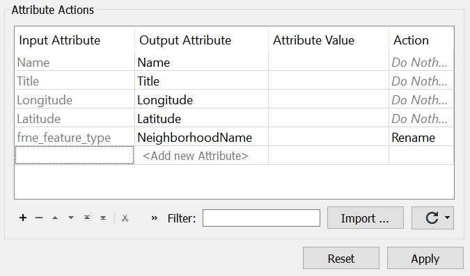
Click OK/Apply.
4) Add Writer Feature Type for Public Art
Now we need a writer feature type for our public art points.
| TIP |
| Remember, we already have our geodatabase writer set up. We don't want to add another writer, because we want all of our data to be written to the same output database. Instead, we need to use feature types, because we want our data to be organized by layer. |
We can add a feature type to a writer in the menu bar under Writers > Add Feature Type. Because we only have one writer it will automatically be selected. Name your new feature type PublicArt and give it Geometry type geodb_point. Your Feature Type dialog should look like this:
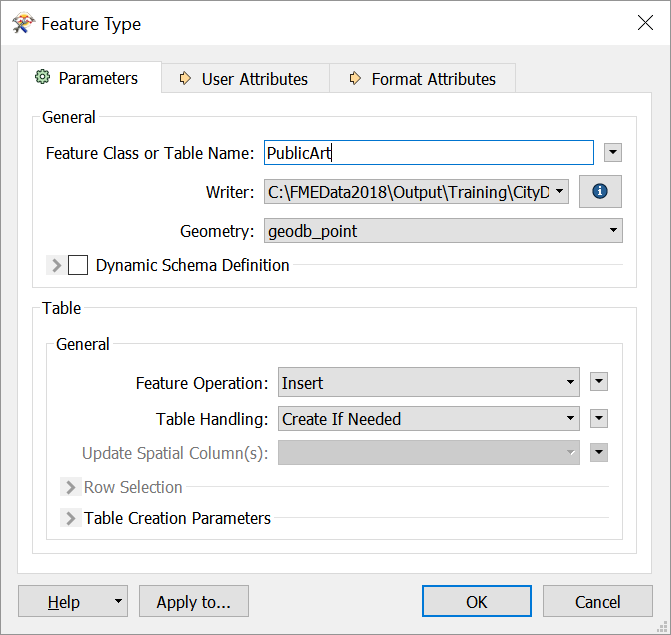
Click OK. Connect your new feature type to the Output port of your Attribute Manager. Your canvas should look like this:
5) Add Shapefile Reader
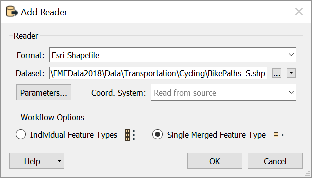
Add another reader by clicking Readers > Add Reader, or by clicking an empty space on the canvas and typing the name or file extension of the format you wish to add and picking it from the Quick Add Menu. In this case that would be shp for Esri Shapefile.
| Reader Format | Esri Shapefile |
| Reader Datasets | C:\FMEData2018\Data\Transportation\Cycling\BikePaths_L.shp C:\FMEData2018\Data\Transportation\Cycling\BikePaths_M.shp C:\FMEData2018\Data\Transportation\Cycling\BikePaths_S.shp |
When you select your dataset, use Ctrl or Shift click to select all three bike path shapefiles.
The bike path data is split up into three shapefiles by length of the bike path (L for long, M for medium, and S for short). Just like the public art points, we don't need these features separated in our database. Therefore, let's change Workflow Options from Individual Feature Types to Single Merged Feature Type. Because shapefiles contain coordinate system information, we don't need to change that here. Your dialog should look like this:
Click OK. This adds another <All> feature type to our canvas. Again, we should add an annotation so it is clear which reader is which:
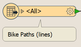
If you inspect the reader feature type you'll find the data already has a PathType attribute with values S, M, or L. Therefore, we don't need to use AttributeManager to rename fme_feature_type like we did for the public art data. However, we also don't want fme_feature_type to be written to our final data.
We can unexpose it on our reader feature type. Select your bike paths reader feature type and go to the Format Attributes tab in the Parameter Editor. You'll see that fme_feature_type is checked. Simply uncheck it and click OK/Apply:
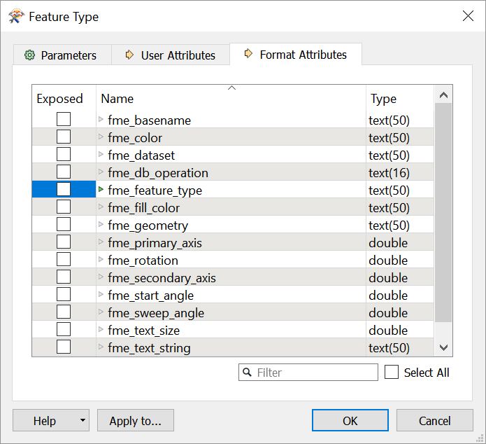
Now if you click the drop-down arrow on your bike paths reader feature type you'll see that fme_feature_type has been removed from the schema as we wanted.
6) Add Writer Feature Type for Bike Paths
Now we need a writer feature type for our bike path lines. Click Writers > Add Feature Type, name your new feature type BikePaths, and give it Geometry type geodb_polyline. Your Feature Type dialog should look like this:
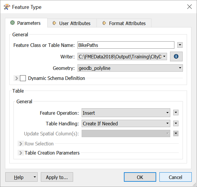
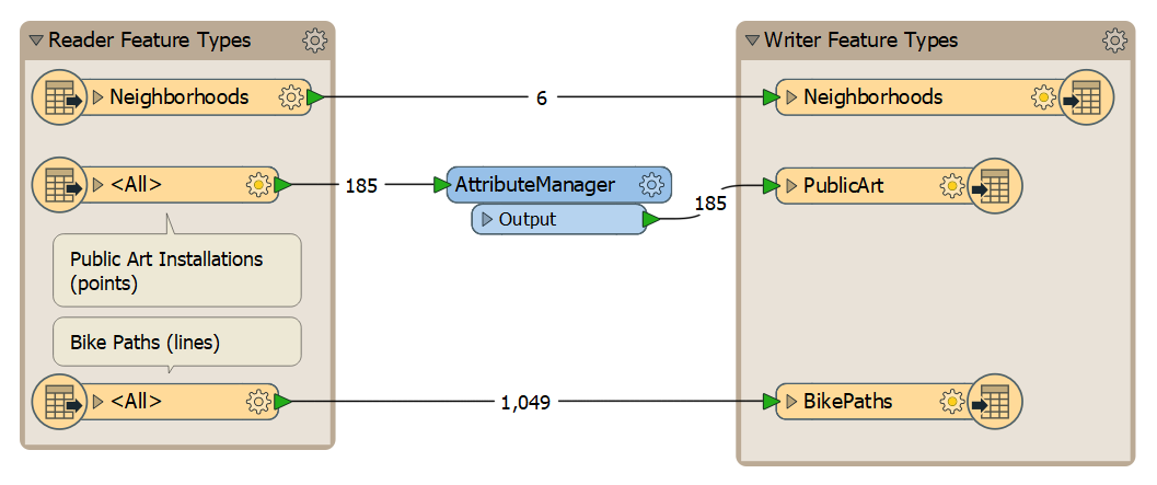
Click OK. Connect your ALL reader feature type containing the bike path features to your writer feature type BikePaths. Your canvas should look like this:
7) Reproject Data
Add a Reprojector transformer to the canvas and then connect it to the Neighborhoods feature type. Choose UTM83-10 as the Destination Coordinate System. Right-click the Reprojector transformer and select Duplicate to add another. Connect this between your AttributeManager output port and your Public Art writer feature type.
This will ensure our neighborhoods and public art data is in the same projection as our bike paths. Your canvas should look like this:
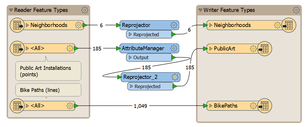
8) Inspect Output
Let's take a look at our data integrated into one geodatabase. You can run your workspace and then open the resulting geodatabase in Data Inspector, or you can click Writers > Redirect to Data Inspector.
When this function is on no data is actually written; instead the results of your translation are sent directly to the Data Inspector. It is useful for checking the results of your translation while your workspace is still in development.
You should see all three layers displayed in Data Inspector, now all stored in the same format in a centralized database:
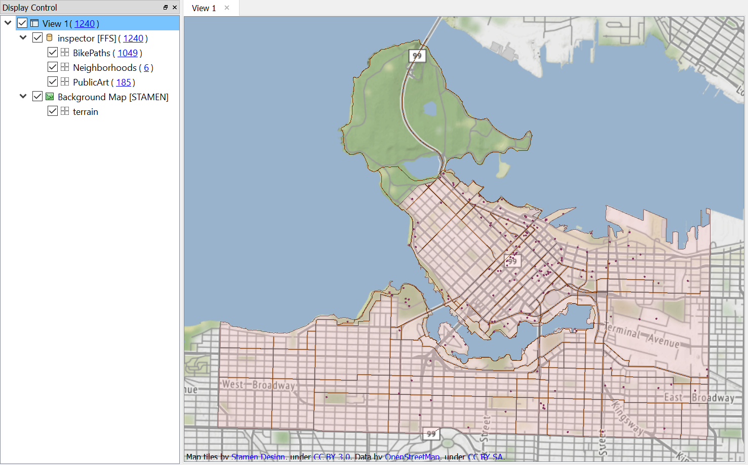
Map tiles by Stamen Design, under CC-BY-3.0. Data by OpenStreetMap, under CC-BY-SA.
9) Example Data Integration Analysis
Let's look at an example of how integrating data facilitates analysis.
What if the City Planning Department wanted to know the total length of bike paths and number of public art installations by neighborhood? How would we do this using this workspace?
Take a minute and write or draw out how you would tackle this problem using what you have learned so far. Don't worry if you can't remember the exact name of transformers. Instead focus on outlining the process you would undertake to perform this analysis.
Let's find out if you were right! Note that there are usually multiple ways to solve a problem in FME, so your solution might still be valid.
Here are the steps we will take to conduct this analysis:
- Sum the total of bike path lengths by neighborhood.
- Sum the count of public art installations by neighborhood.
- Output a table or chart to show the results.
Let's walk through how to do that in Workbench.
10) Calculate Statistics for Public Art
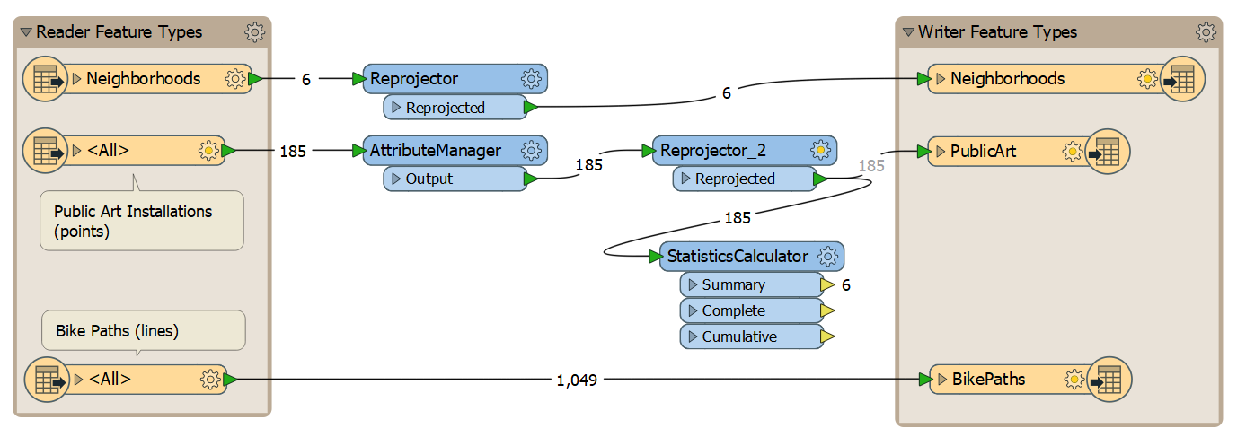
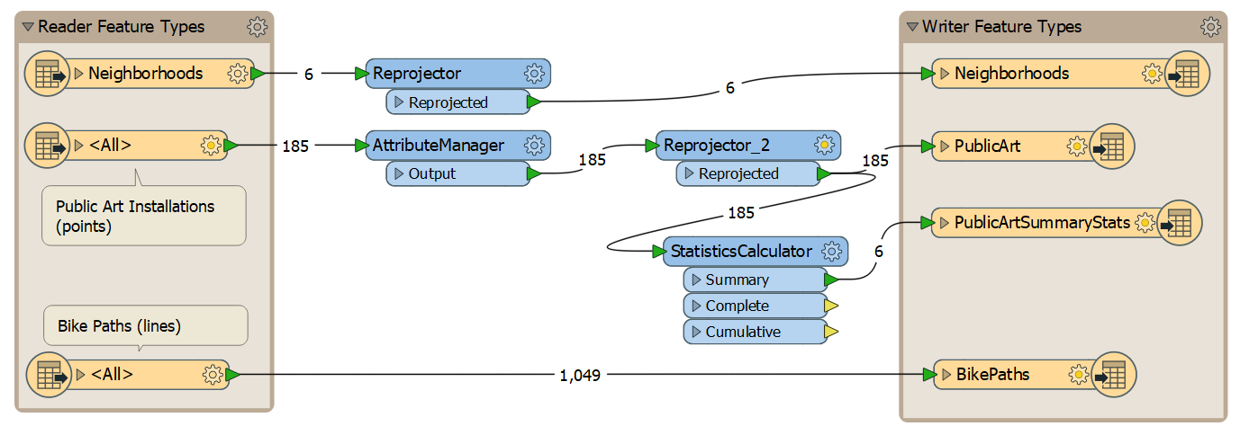
Add a StatisticsCalculator after your public art Reprojector. We will use this to count the number of public art installations by neighborhood. Your canvas should look like this:
Open the parameters for the StatisticsCalculator. Select any attribute for Attributes to Analyze (it is just counting if there is a value, so any attribute will do). With the exception of Total Count Attribute, clear all the boxes in Calculate Attributes so they are not generated. Finally, set Group By to NeighborhoodName. Your dialog should look like this:
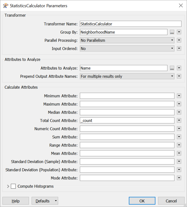
Click OK/Apply. The Summary output port will now output a table with the count of public art installations by neighborhood.
Let's write that out as a table in our geodatabase. Click Writers > Add Feature Type. Call it PublicArtSummaryStats and give it Geometry type geodb_no_geom. This will store it without geometry as a table. Click Ok. Once your new feature type is added, connect it to the Summary port of your StatisticsCalculator. Your canvas should look like this:
You can run the translation and inspect the table if you want.
11) Calculate Statistics for Bike Paths
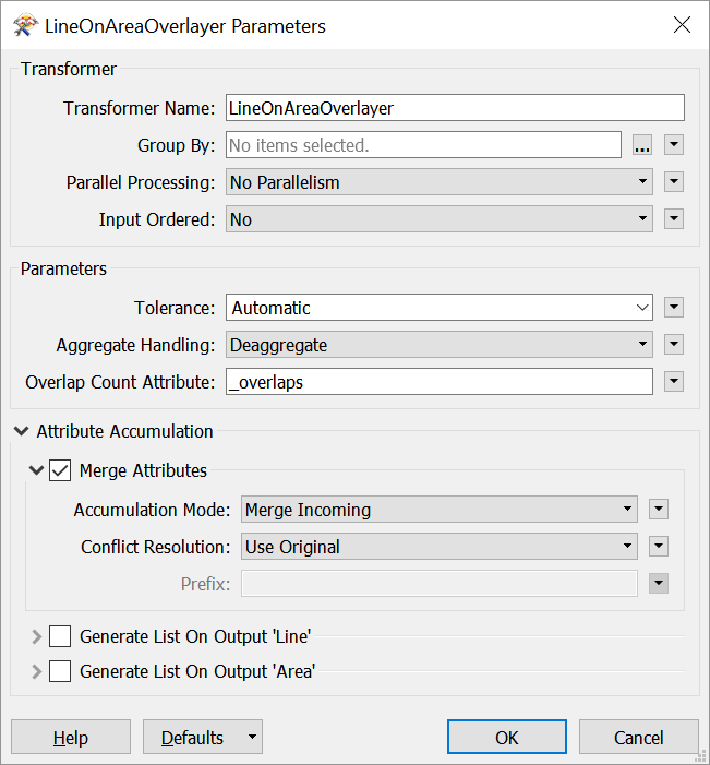
Add a LineOnAreaOverlayer to your canvas. This transformer will let us add attributes from the neighborhoods to the bike paths that overlap them. This will let us know which neighborhood each bike path segment is in. The Reprojector should connect to the Area port (because it is polygons of neighborhoods) and the bike path reader feature type should connect to the Line port. Open the LineOnAreaOverlayer parameters and check the box Attribute Accumulation > Merge Attributes. Your dialog should look like this:
Click OK/Apply.
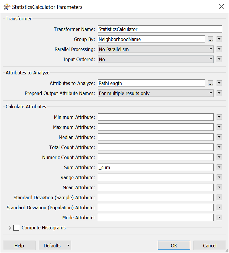
Now let's add a StatisticsCalculator to the Line output port of the LineOnAreaOverlayer. We will use this to sum up the PathLength for each feature and report the total length of bike paths, by neighborhood. To do this, open the paramters for the StatisticsCalculator. Set Group By to NeighborhoodName. Set the Attributes to Analyze to PathLength. With the exception of Sum Attribute, clear all the boxes in Calculate Attributes so they are not generated. Your dialog should look like this:
Click OK/Apply.
If you inspect the results of this transformer (using Feature Caching), you'll find that one of the neighborhood names is blank. This is because there is no neighborhood polygon for the bike paths in Stanley Park, the large park northwest of Vancouver's downtown. Let's fix this in the output table.
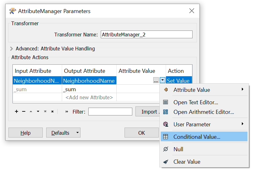
Add an AttributeManager and connect it to the StatisticsCalculator Summary output port. Open its parameters and click the drop-down arrow in the Attribute Value column for the Input Attribute NeighborhoodName. Then select Conditional Value:
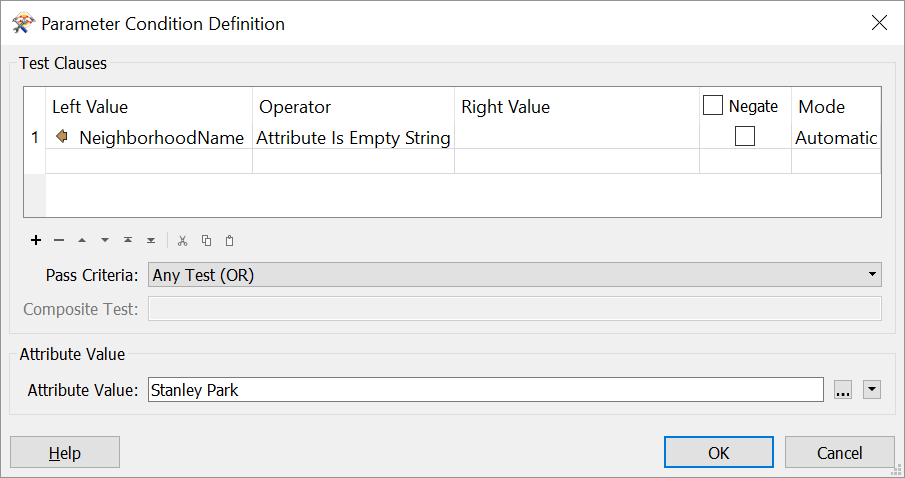
We will set the AttributeManager to set the value of NeighborhoodName to Stanley Park if it doesn't already have a value. Double click on the cell in the row If and the column Test Condition. In the new window, for Left Value select the attribute NeighborhoodName. For the Operator Select Attribute is Empty String. Finally, under Attribute Value > Attribute Value, enter Stanley Park. Your dialog will look like this:
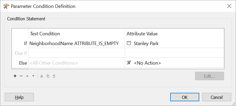
Click OK. Now your Parameter Condition Definition should look like this:
Click OK again. Now your Attribute Manager will look like this:
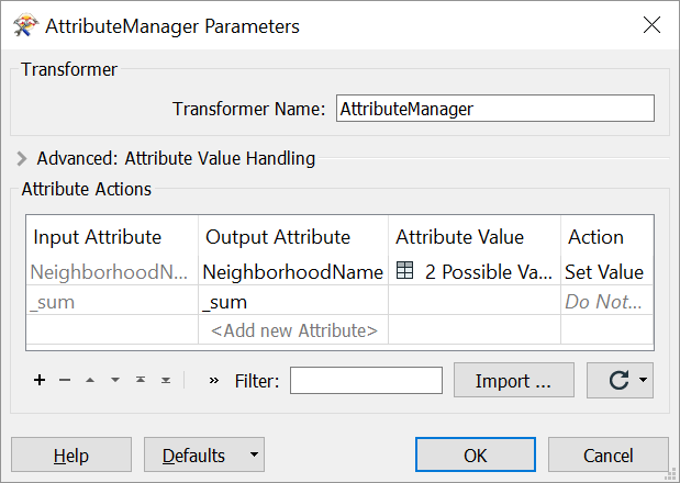
Great! Now our AttributeManager will take care of that empty NeighborhoodName value and replace it with Stanley Park.
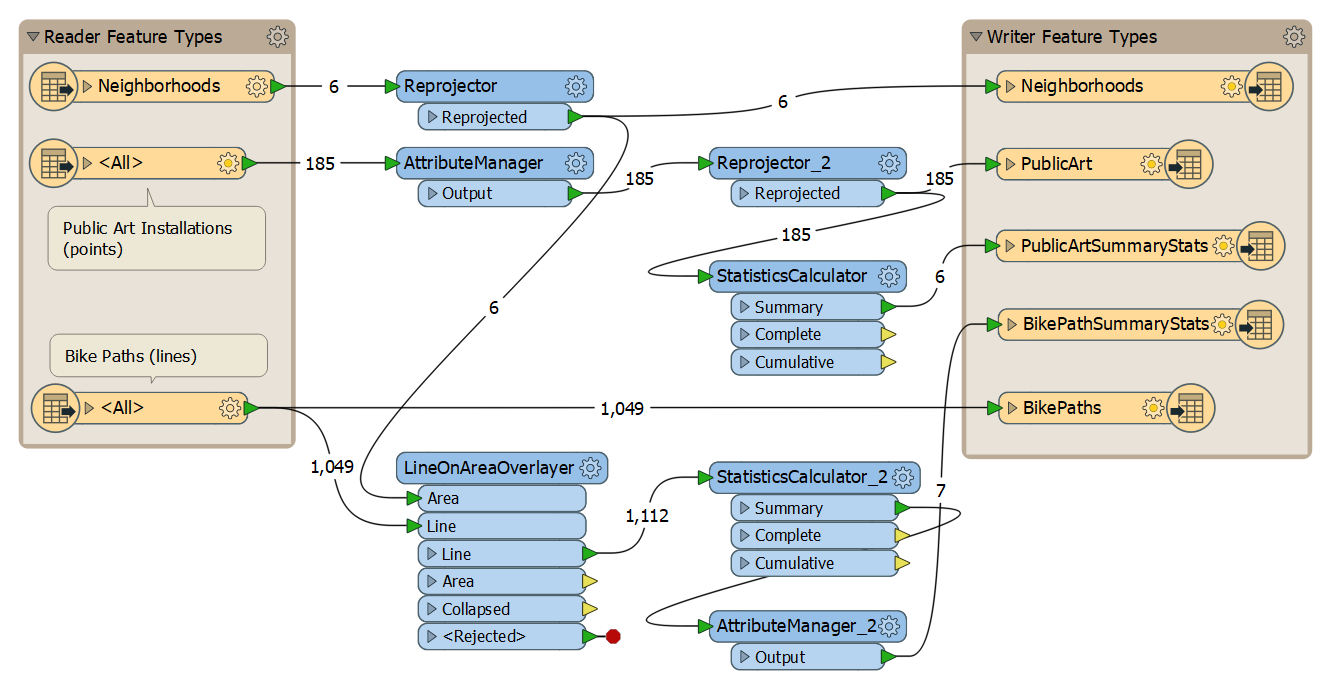
Let's write these results as a table in our geodatabase as well. Click Writers > Add Feature Type. Call it BikePathSummaryStats and give it Geometry type geodb_no_geom. Click Ok. Once your new feature type is added, connect it to the Summary port of your bike paths StatisticsCalculator. Your canvas should look like this:
You can run the translation and inspect the table if you want. Note the presence of the new Stanley Park value.
12) Create Charts
Finally, lets create two charts to summarize our findings.
Add a ChartGenerator transformer to the canvas. Attach it to the Summary output port of your public art StatisticsCalculator. Open its parameters. Under Chart Settings, for Type select Pie. For Title enter: Distribution of public art by neighborhood, Vancouver, BC. Under Data Series, set the Data Attribute to _count and the Label Attribute to NeighborhoodName. Change Show Percentages to Yes. Your dialog should look like this:
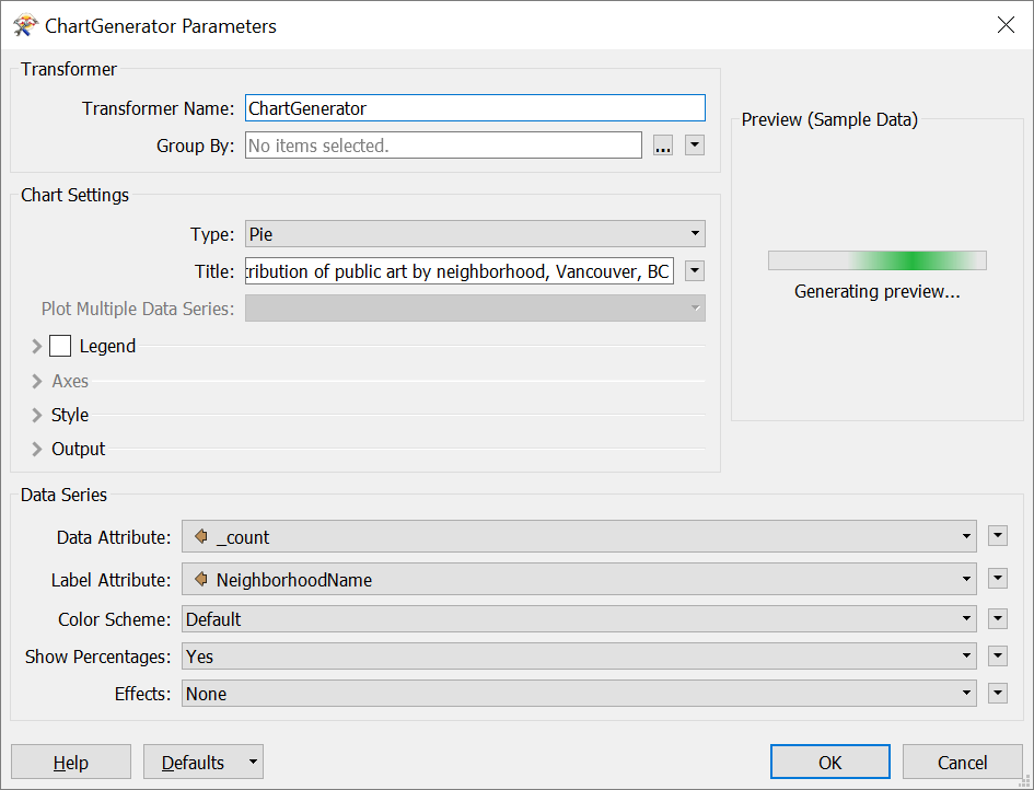
| TIP |
| If you want to change the order the neighborhoods are displayed in for this or the bike paths chart, add a Sorter transformer before the ChartGenerator. |
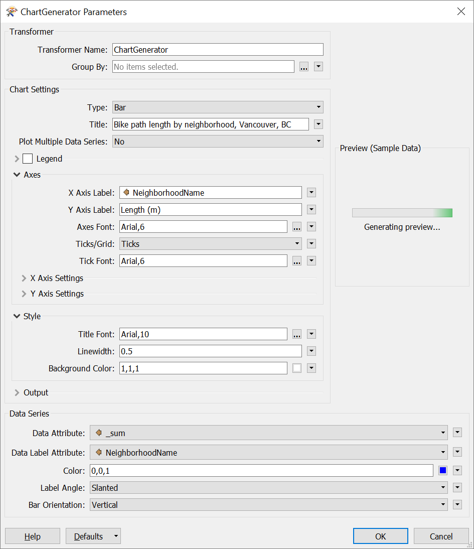
Add another ChartGenerator to the canvas, this time connected to the Summary output port of your bike paths StatisticsCalculator. Let's make this chart type Bar and title it: Bike path length by neighborhood, Vancouver, BC. Change the following parameters:
- Axes | X Axis Label: NeighborhoodName
- Axes | Y Axis Label: Length (m)
- Axes | Axes Font: Arial, 6
- Axes | Tick Font: Arial, 6
- Style | Title Font: Arial, 10
- Data Series | Data Attribute: _sum
- Data Series | Data Label Attribute: NeighborhoodName
This will generate a chart that shows the total length of bike paths in each neighborhood. Your dialog should look like this:
Click OK/Apply.
13) Write Charts to PNGs
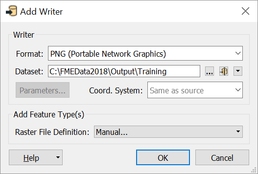
Now let's hook these ChartGenerators up to writers so we can write the charts as images. Click Writers > Add Writer and use the following parameters:
| Writer Format | PNG (Portable Network Graphics) |
| Writer Dataset | C:\FMEData2018\Output\Training |
For Add Feature Type(s) > Raster File Definition, choose Manual. We are choosing this because we don't want these chart images to map any schemas that already exist in our workspace. The dialog should look like this:
Click OK.
Another dialog will open to specify a feature type for our PNG writer. For Raster File Name enter PublicArtChart. Change Raster > World File Generation to No. Your dialog should look like this:

Click OK. Now connect your new writer feature type to the Output port of your public art ChartGenerator.
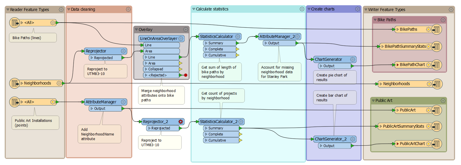
Repeat this process for a new feature type named BikePathChart: click Writers > Add Writer(s) and ensure Writer is set to PNGRASTER. Connect that to the bike path ChartGenerator. Since this is as far as we'll be going in this example, add bookmarks and/or annotations to explain your workspace (see the Style section if you need a reminder how to do this). After that your canvas should look something like this:
| CONGRATULATIONS |
By completing this exercise you have learned how to:
|
Now that you have some practice integrating data, it's your turn! Use the skills you gained in the previous exercises to add one more dataset to the workspace to answer a question or solve a problem.
Here are some example questions:
- How many addresses (C:\FMEData2018\Data\Addresses\Addresses.gdb) are within 100 meters of a bike path?
- Hint: use the Bufferer and PointOnAreaOverlayer transformers. Don't forget to make sure all your data shares a coordinate system before analyzing it.
- Where could the city locate a new public art installation? First find out which neighborhood has the fewest public art installations. Then find a city-owned property (C:\FMEData2018\Data\Parcels\CityProperties\CityProperties.shp) in that neighborhood that is the furthest away from existing public art installations. This is the site for a new installation.
- Hint: use the Sorter, Tester, PointOnAreaOverlayer, NeighborFinder (check out the _distance attribute), and Sampler (check out Sampling Type: First N Features) transformers.
- Do any city parks (C:\FMEData2018\Data\Parks\Parks.tab) not have access to bike lanes? If so, which ones? If not, which have the best and worse access?
- Hint: use the Bufferer, LineOnAreaOverlayer, and/or NeighborFinder.
As a reminder, please refer to your lab requirements.
The next section contains optional advice on some of the procedures you may have to carry out depending on the data you choose.
Finally, don't forget to answer your lab questions.