| Exercise 2a | Flood Risk Project: Simple Filtering Method |
| Start Workspace | C:\FMEData2018\Workspaces\DesktopAdvanced\Attributes-Ex2-Begin.fmw |
| End Workspace | C:\FMEData2018\Workspaces\DesktopAdvanced\Attributes-Ex2a-Complete.fmw |
This simple filtering method is a two-step process involving an AttributeFilter and several AttributeRangeMapper transformers. You should already have the start workspace open.
1) Place AttributeFilter
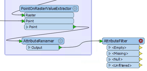
Place an AttributeFilter connected to the AttributeRenamer:
Inspect the parameters either in the parameters dialog or the Parameter Editor window. Select Zone as the attribute to filter by. In the Attribute Values field enter the values 100, 200, and 300:
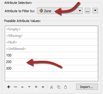
You could use the Import function, but for so few values it’s hardly worth it.
Apply the changes, and you’ll see a new output port added for each value you specified.
2) Add AttributeRangeMapper
Add an AttributeRangeMapper transformer and connect it to the 100 output port of the AttributeFilter:

Inspect the parameters. As you’ll see this is a lookup table that involves ranges. We should be able to map the elevation range to a final flood risk using the information in the original table.
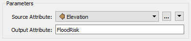
So, select Elevation as the Source Attribute. Enter FloodRisk as the Output Attribute:
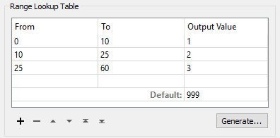
In the Range Lookup Table, enter the From-To values as follows:
| From | To | Output Value |
|---|---|---|
| 0 | 10 | 1 |
| 10 | 25 | 2 |
| 25 | 60 | 3 |
If an elevation falls precisely on one value (for example 25), it is counted in the lower band (i.e. 10-25). Enter 999 as the Default, so that any features whose elevation does not match, for whatever reason, is flagged appropriately:
Apply the changes. You may wish to run the translation and inspect the AttributeRangeMapper results, to ensure that this part is working correctly.
| Miss Vector says... |
| Hopefully you see that the Output Value numbers come from the flood risk table in the introduction to this exercise! Here we're combining the zone that we just filtered by (zone 100) with each possible risk value. |
3) Duplicate AttributeRangeMapper
Now we need to do the same thing for each of the other AttributeFilter output ports. Rather than set them up manually – as above – the easiest method is to copy the AttributeRangeMapper transformer that we just set up.
So, click on the existing AttributeRangeMapper and press Ctrl+D to duplicate it. Repeat and connect each duplicate to a different AttributeFilter output port.
The workspace will now look like this:
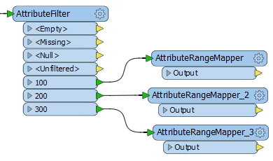
Now open the parameters dialog for each of the new AttributeRangeMapper transformers in turn and set up the correct Output Values in accordance with the original table of calculations.
The Output Values will be:
| 100m Zone | 1 | 2 | 3 |
| 200m Zone | 2 | 3 | 4 |
| 300m Zone | 3 | 4 | 5 |
4) Add Inspector
Inspecting cached data doesn't allow you to separate that data out for easier inspection. So place a single Inspector transformer and connect each AttributeRangeMapper output to it.
Open the Inspector parameters dialog and under Group-By select the newly created attribute called FloodRisk.
| TIP |
| To achieve the same effect with Feature Caching, add a second AttributeFilter and filter by FloodRisk. Set the filters to 1,2,3,4,5. Then run the workspace, select the transformer, and press Ctrl+I to inspect it. |
5) Save and Run Workspace
Save your workspace as a new file to preserve the starting workspace and then run it. You should see each address colored to match its flood risk. You can also turn off each zone, in turn, to see which addresses are most/least at risk.
| Professor Lynn Guistic says… |
| If you’re sharp today, you’ll have noticed you could do this process in the reverse order. Instead of filtering by zone then mapping elevation, you could filter by elevation and then map zone. This would require a combination of AttributeRangeFilter and AttributeValueMapper transformers. |
| CONGRATULATIONS |
By completing this exercise you have learned how to:
|